Experiments#
This section presents the experiments performed to analyze the different aspects of the parallel Poisson solver. The experiments build chronologically towards a final ‘integration’ test where we verify the correctness of our implementation and finally a scaling analysis.
01 - Choice of Kernel: NumPy vs Numba#
Description#
Here we compare Numba JIT-compiled kernels vs pure NumPy implementations. This experiment tests only the computational kernel in isolation - without MPI, domain decomposition, or parallel communication.
Purpose#
Identify impacts of the choice of kernel implementations and parameters like thread-count.
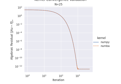
Kernel correctness - Verify both implementations produce identical results
Performance pr. iteration - Compare execution time for NumPy vs Numba with different thread counts across various problem sizes
Speedup analysis - Comparing different Numba thread configurations against a NumPy baseline.
Compute time scaling - Measure computation cost with fixed iteration count and also fixed tolerance.
Decision Point: Choose optimal kernel (NumPy or Numba) and thread count for subsequent experiments.

02 - Domain Decomposition#
Description#
Compare 1D sliced decomposition and 3D cubic decomposition strategies for parallel domain partitioning. This experiment tests domain decomposition logic - partitioning across MPI ranks, local to global indice mapping, and how ghost zones are structured.
Sliced (1D): Splits domain along Z-axis with horizontal slices, exchanging 2 ghost planes.
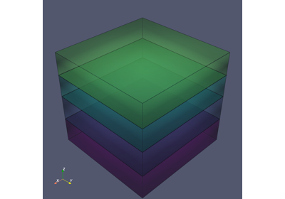
Cubic (3D): Uses 3D Cartesian grid across all dimensions, exchanging 6 ghost faces.
Purpose#
Determine which decomposition strategy provides better performance for different problem sizes and rank counts by analyzing: Get an understanding of how the type of domain decomposition impacts the size of the data that needs to be communicated between ranks along with the ‘connectivity’ of different ranks.
Visual comparison - Illustrate how the domain is partitioned for each method
Surface-area-to-volume ratios - investigate how much data needs to be communicated between ranks depending on the decomposition strategy
03 - Communication Methods#
Description#
Compare custom MPI datatypes vs NumPy array communication for halo exchange operations. This experiment tests communication implementation details - how data is transferred between ranks during halo exchanges.
Custom MPI Datatypes: Zero-copy communication using MPI.Create_contiguous() and MPI.Create_subarray().
NumPy Arrays: Explicit buffer copies using np.ascontiguousarray().
Purpose#
Determine whether custom MPI datatypes provide measurable performance improvements over NumPy arrays by evaluating:
Communication overhead - Demonstrate whether custom datatypes reduce overhead compared to NumPy arrays
Scaling behavior - Analyze how each method scales with problem size and rank count
Scaling order analysis - Use log-log plots with reference lines to derive computational complexity
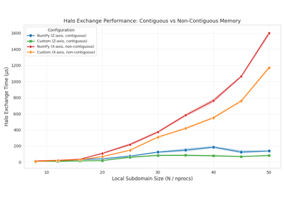
Communication Analysis: Contiguous vs Non-Contiguous

04 - Solver Validation#
Description#
End-to-end validation of the complete Poisson solver across all implementation permutations. This experiment tests the fully assembled solver - Decomposition from experiment 02, and communication from experiment 03.
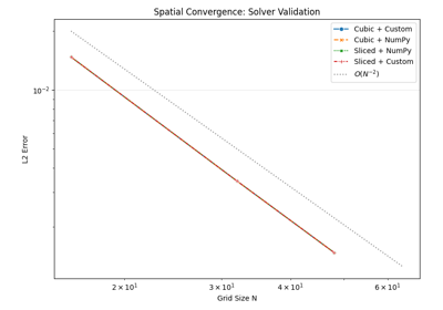
The correctness is asserted by comparing the obtained solution with the analytical solution in a grid refinement study and verifying the theoretical order of spatial accuracy.
Note
We only use a single kernel-configuration here since the kernel correctness has already been established in experiment 01.
Purpose#
Establish correctness of the solver implementation by:
Analytical comparison - Test against known exact solution:
u(x,y,z) = sin(πx)sin(πy)sin(πz)Spatial convergence - Demonstrate expected O(h²) convergence order as grid is refined

05 - Scaling Analysis#
Description#
Scaling analysis using the validated solver configuration from experiment 04. This experiment measures the performance limits of the complete solver across different problem sizes and processor counts.
Strong Scaling: Fixed problem size with increasing ranks → measures parallel speedup.
Weak Scaling: Constant work per rank with proportional growth → measures scalability.
Purpose#
Characterize the parallel performance limits of the validated solver by analyzing:
Strong scaling efficiency - Measure speedup curves for fixed problem sizes with increasing processor counts
Weak scaling efficiency - Evaluate performance with constant work per rank as both problem size and processors grow
Memory usage scaling - Analyze per-rank memory footprint and total memory requirements as problem size and rank count vary
Parallel I/O considerations - Demonstrate impact of parallel HDF5 writes vs serial gather-to-rank-0 on scaling behavior