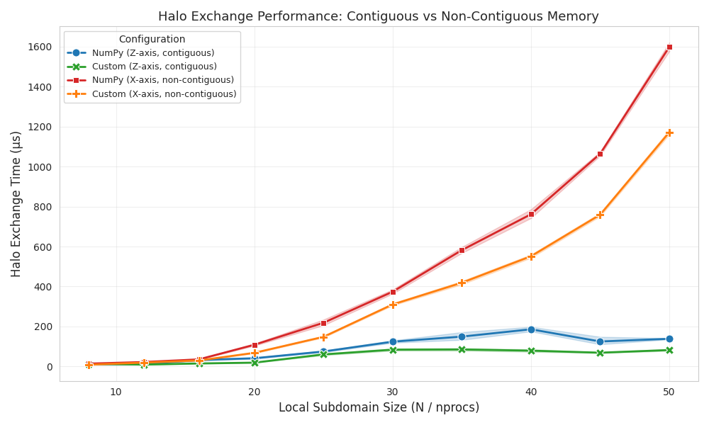
Communication Analysis: Contiguous vs Non-Contiguous

Compares NumPy array copies vs MPI custom datatypes for halo exchange, demonstrating the benefit of zero-copy communication for non-contiguous data.

Uses per-iteration timeseries data for tight confidence intervals.

import matplotlib.pyplot as plt
import pandas as pd
import seaborn as sns

from Poisson import get_project_root

Setup

sns.set_style("whitegrid")
plt.rcParams["figure.dpi"] = 100

repo_root = get_project_root()
data_dir = repo_root / "data" / "communication"
fig_dir = repo_root / "figures" / "communication"
fig_dir.mkdir(parents=True, exist_ok=True)

Load Data

parquet_files = list(data_dir.glob("communication_*.parquet"))
if not parquet_files:
    raise FileNotFoundError(
        f"No data found in {data_dir}. Run compute_communication.py first."
    )

df = pd.concat([pd.read_parquet(f) for f in parquet_files], ignore_index=True)

print(f"Loaded {len(df)} per-iteration measurements")
print(f"Configurations: {df['label'].unique()}")
print(f"Problem sizes: {sorted(df['N'].unique())}")

Loaded 20000 per-iteration measurements
Configurations: ['NumPy (Z-axis, contiguous)' 'Custom (Z-axis, contiguous)'
 'NumPy (X-axis, non-contiguous)' 'Custom (X-axis, non-contiguous)']
Problem sizes: [np.int64(32), np.int64(48), np.int64(64), np.int64(80), np.int64(100), np.int64(120), np.int64(140), np.int64(160), np.int64(180), np.int64(200)]

Halo Exchange Time vs Problem Size

Shows all 4 configurations with 95% CI from per-iteration data

fig, ax = plt.subplots(figsize=(10, 6))

palette = {
    "NumPy (Z-axis, contiguous)": "#1f77b4",
    "Custom (Z-axis, contiguous)": "#2ca02c",
    "NumPy (X-axis, non-contiguous)": "#d62728",
    "Custom (X-axis, non-contiguous)": "#ff7f0e",
}

sns.lineplot(
    data=df,
    x="local_N",
    y="halo_time_us",
    hue="label",
    style="label",
    markers=True,
    dashes=False,
    palette=palette,
    ax=ax,
    errorbar=("ci", 95),
    markersize=8,
    linewidth=2,
)

ax.set_xlabel("Local Subdomain Size (N / nprocs)", fontsize=12)
ax.set_ylabel("Halo Exchange Time (μs)", fontsize=12)
ax.set_title(
    "Halo Exchange Performance: Contiguous vs Non-Contiguous Memory", fontsize=13
)
ax.legend(title="Configuration", fontsize=9, loc="upper left")
ax.grid(True, alpha=0.3)

plt.tight_layout()
output_file = fig_dir / "communication_comparison.pdf"
plt.savefig(output_file, bbox_inches="tight")
print(f"Saved: {output_file}")
plt.show()

Saved: /home/runner/work/LSM-P2/LSM-P2/figures/communication/communication_comparison.pdf

Summary Statistics

print("\n" + "=" * 70)
print("Summary: Mean halo time (μs) with 95% CI by local subdomain size")
print("=" * 70)
summary = df.groupby(["local_N", "label"])["halo_time_us"].agg(["mean", "std", "count"])
summary["ci95"] = 1.96 * summary["std"] / (summary["count"] ** 0.5)
summary["display"] = summary.apply(
    lambda r: f"{r['mean']:.1f} ± {r['ci95']:.1f}", axis=1
)
print(summary["display"].unstack().to_string())

======================================================================
Summary: Mean halo time (μs) with 95% CI by local subdomain size
======================================================================
label   Custom (X-axis, non-contiguous) Custom (Z-axis, contiguous) NumPy (X-axis, non-contiguous) NumPy (Z-axis, contiguous)
local_N
8                             8.2 ± 0.1                  12.7 ± 1.8                     13.8 ± 0.8                 10.6 ± 1.3
12                           18.8 ± 0.6                   8.8 ± 0.4                     21.9 ± 0.5                 11.3 ± 0.4
16                           29.7 ± 1.0                  14.7 ± 1.0                     35.2 ± 1.5                 32.3 ± 4.8
20                           67.8 ± 2.8                  18.7 ± 1.2                    108.2 ± 5.6                 40.7 ± 3.6
25                          147.8 ± 3.9                  59.9 ± 4.8                   218.2 ± 14.2                 74.5 ± 4.0
30                          310.0 ± 5.4                  83.8 ± 5.4                   373.7 ± 10.4                123.6 ± 5.9
35                          418.7 ± 8.4                  84.7 ± 6.7                   581.8 ± 15.3               149.0 ± 20.9
40                          551.2 ± 8.6                  78.8 ± 6.5                   761.4 ± 23.2               185.7 ± 11.7
45                          759.2 ± 8.3                  68.6 ± 2.2                  1064.0 ± 10.1               124.7 ± 19.8
50                        1171.9 ± 11.5                  81.7 ± 4.9                  1599.3 ± 22.5                138.1 ± 2.9