Validation Analysis and Visualization

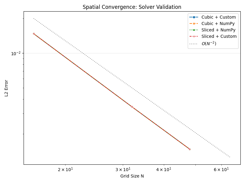
1. Analyze and visualize spatial convergence for solver validation

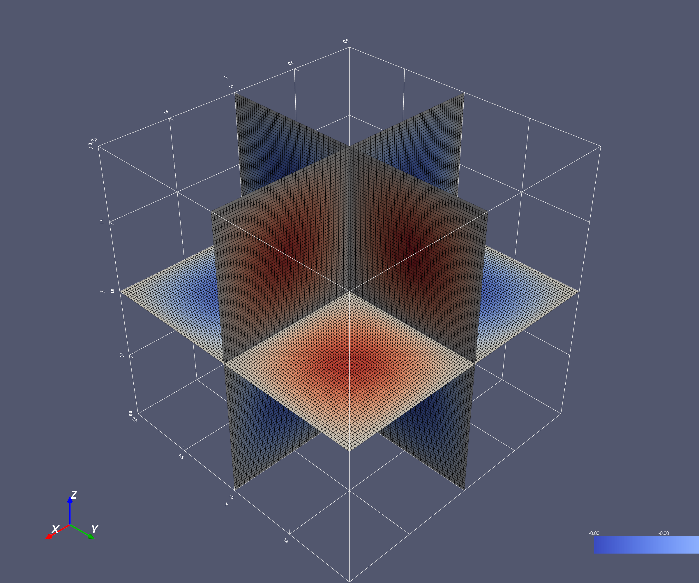
2. Generate 3D visualization of analytical solution

Verifies O(h²) = O(N⁻²) convergence by comparing numerical solutions against the analytical solution u(x,y,z) = sin(πx)sin(πy)sin(πz).

Loaded 12 validation results
Strategies: ['cubic' 'sliced']
Problem sizes: [np.int64(16), np.int64(32), np.int64(48)]

============================================================
PART 2: 3D Solution Visualization
============================================================
Saved: /home/runner/work/LSM-P2/LSM-P2/figures/validation/solution_3d.png

import matplotlib.pyplot as plt
import numpy as np
import pandas as pd
import seaborn as sns
import pyvista as pv

from Poisson import get_project_root

# ============================================================================
# Setup
# ============================================================================

# Matplotlib setup
sns.set_style()

# PyVista setup
pv.set_plot_theme("paraview")

# Get paths using installed package utility (works in Sphinx-Gallery)
repo_root = get_project_root()
data_dir = repo_root / "data" / "validation"
fig_dir = repo_root / "figures" / "validation"
fig_dir.mkdir(parents=True, exist_ok=True)

# ============================================================================
# Part 1: Convergence Analysis
# ============================================================================
# Load validation data from HDF5 files
h5_files = list(data_dir.glob("*.h5"))
if not h5_files:
    raise FileNotFoundError(
        f"No data found in {data_dir}. Run compute_validation.py first."
    )

df = pd.concat([pd.read_hdf(f, key="results") for f in h5_files], ignore_index=True)

print(f"\nLoaded {len(df)} validation results")
print(f"Strategies: {df['decomposition'].unique()}")
print(f"Problem sizes: {sorted(df['N'].unique())}")

# Create labels for plotting
df["Strategy"] = df["decomposition"].str.capitalize()
df["Communicator"] = (
    df["communicator"]
    .str.replace("haloexchange", "")
    .str.replace("custom", "Custom")
    .str.replace("numpy", "NumPy")
)
df["Method"] = df["Strategy"] + " + " + df["Communicator"]

# Use lineplot (single rank count = 8)
fig, ax = plt.subplots(figsize=(8, 6))

sns.lineplot(
    data=df,
    x="N",
    y="final_error",
    hue="Method",
    style="Method",
    markers=True,
    dashes=True,
    ax=ax,
)

# Add O(N^-2) reference line
N_ref = [16, 64]
ax.plot(N_ref, [0.02, 0.02 * (16 / 64) ** 2], "k:", alpha=0.5, label=r"$O(N^{-2})$")

ax.set_xscale("log")
ax.set_yscale("log")
ax.grid(True, alpha=0.3)
ax.set_xlabel("Grid Size N")
ax.set_ylabel("L2 Error")
ax.set_title("Spatial Convergence: Solver Validation")
ax.legend()

fig.tight_layout()
output_file = fig_dir / "validation_convergence.pdf"
fig.savefig(output_file)

# ============================================================================
# Part 2: 3D Solution Visualization
# ============================================================================

print("\n" + "=" * 60)
print("PART 2: 3D Solution Visualization")
print("=" * 60)

# Generate analytical solution at high resolution
N = 100
x = np.linspace(0, 2, N)
y = np.linspace(0, 2, N)
z = np.linspace(0, 2, N)
X, Y, Z = np.meshgrid(x, y, z, indexing="ij")
u_analytical = np.sin(np.pi * X) * np.sin(np.pi * Y) * np.sin(np.pi * Z)

# Create structured grid
grid = pv.StructuredGrid(X, Y, Z)
grid["solution"] = u_analytical.flatten(order="F")


# Create orthogonal slices at domain center
slices = grid.slice_orthogonal(x=1.0, y=1.0, z=1.0)

# Create single view plotter
plotter = pv.Plotter(off_screen=True, window_size=[2400, 2000])

# Add orthogonal slices
plotter.add_mesh(
    slices,
    scalars="solution",
    cmap="coolwarm",
    show_edges=True,
    edge_color="black",
    line_width=0.5,
    show_scalar_bar=True,
    scalar_bar_args={
        "title": "u(x,y,z)",
        "position_x": 0.85,
        "position_y": 0.05,
        "title_font_size": 20,
        "label_font_size": 16,
        "fmt": "%.2f",
        "n_labels": 7,
    },
)

# Add coordinate axes
plotter.add_axes(
    interactive=False,
    line_width=5,
    x_color="red",
    y_color="green",
    z_color="blue",
    xlabel="X",
    ylabel="Y",
    zlabel="Z",
)

# Add bounds with labels
plotter.show_bounds(
    grid="back",
    location="outer",
    xtitle="X",
    ytitle="Y",
    ztitle="Z",
    font_size=12,
    all_edges=True,
)

# Show the plot (Sphinx-Gallery scraper will capture it)
# Also save a copy to figures directory
output_file = fig_dir / "solution_3d.png"
plotter.screenshot(output_file, transparent_background=True)
print(f"Saved: {output_file}")
plotter.show()