Visualization of Kernel Experiments

Comprehensive analysis and visualization of NumPy vs Numba kernel benchmarks.

import pandas as pd
import matplotlib.pyplot as plt
import seaborn as sns

from Poisson import get_project_root

Setup

sns.set_theme()

# Get paths using installed package utility (works in Sphinx-Gallery)
repo_root = get_project_root()
data_dir = repo_root / "data" / "01-kernels"
fig_dir = repo_root / "figures" / "kernels"
fig_dir.mkdir(parents=True, exist_ok=True)

# Check if data exists
if not list(data_dir.glob("*.parquet")):
    print(f"Data not found: {data_dir}. Run compute_kernels.py first.")
    # Graceful exit for docs build
    import sys

    sys.exit(0)

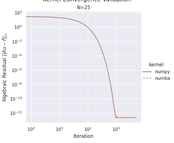
Plot 1: Convergence Validation

convergence_file = data_dir / "kernel_convergence.parquet"
if convergence_file.exists():
    df_conv = pd.read_parquet(convergence_file)

    # Create faceted plot: one subplot per problem size
    g = sns.relplot(
        data=df_conv,
        x="iteration",
        y="physical_errors",
        col="N",
        hue="kernel",
        style="kernel",
        kind="line",
        dashes=True,
        markers=False,
        facet_kws={"sharey": True, "sharex": False},
    )

    g.set(xscale="log", yscale="log")
    g.set_axis_labels("Iteration", r"Algebraic Residual $||Au - f||_\infty$")
    g.set_titles(col_template="N={col_name}")
    g.fig.suptitle(r"Kernel Convergence Validation", y=1.02)

    # Save figure
    g.savefig(fig_dir / "01_convergence_validation.pdf")

Load and Prepare Benchmark Data

benchmark_file = data_dir / "kernel_benchmark.parquet"
df = pd.read_parquet(benchmark_file)

# Convert to milliseconds
df["time_ms"] = df["compute_times"] * 1000

# Prepare configuration labels
df["config"] = df.apply(
    lambda row: "NumPy"
    if row["kernel"] == "numpy"
    else f"Numba ({int(row['num_threads'])} threads)",
    axis=1,
)

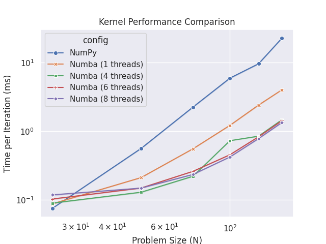
Plot 2: Performance Comparison

# Create plot - seaborn will automatically compute mean and confidence intervals
fig, ax = plt.subplots()
sns.lineplot(
    data=df,
    x="N",
    y="time_ms",
    hue="config",
    style="config",
    markers=True,
    dashes=False,
    errorbar="ci",  # Show confidence intervals
    ax=ax,
)

ax.set_xscale("log")
ax.set_yscale("log")
ax.set_xlabel("Problem Size (N)")
ax.set_ylabel("Time per Iteration (ms)")
ax.set_title("Kernel Performance Comparison")

fig.savefig(fig_dir / "02_performance.pdf")

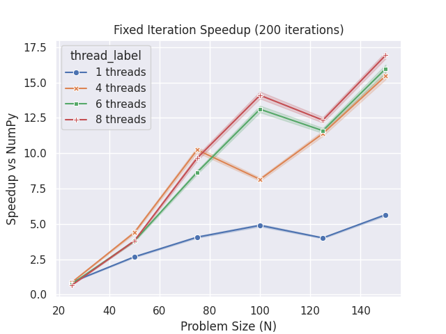
Plot 3: Speedup Analysis

# Compute numpy baseline for each N and iteration
df_numpy = df[df["kernel"] == "numpy"][["N", "iteration", "compute_times"]].rename(
    columns={"compute_times": "numpy_time"}
)
df_speedup = df[df["kernel"] == "numba"].merge(
    df_numpy, on=["N", "iteration"], how="left"
)
df_speedup["speedup"] = df_speedup["numpy_time"] / df_speedup["compute_times"]
df_speedup["thread_label"] = (
    df_speedup["num_threads"].astype(int).astype(str) + " threads"
)

# Create speedup plot - seaborn will compute mean and error bars
fig, ax = plt.subplots()
sns.lineplot(
    data=df_speedup,
    x="N",
    y="speedup",
    hue="thread_label",
    style="thread_label",
    markers=True,
    dashes=False,
    errorbar="ci",
    ax=ax,
)

ax.set_xlabel("Problem Size (N)")
ax.set_ylabel("Speedup vs NumPy")
ax.set_title("Fixed Iteration Speedup (200 iterations)")

fig.savefig(fig_dir / "03_speedup_fixed_iter.pdf")