Lid-Driven Cavity Flow Visualization

This script visualizes the computed lid-driven cavity flow solution and validates the results against the benchmark data from Ghia et al. (1982).

Setup and Load Data

Import visualization utilities and load the computed solution from HDF5 file.

from utils import get_project_root, LDCPlotter, GhiaValidator, plot_validation

# Configuration
Re = 100
N = 64  # Grid size (number of cells)
Re_str = f"Re{int(Re)}"

project_root = get_project_root()
data_dir = project_root / "data" / "FV-Solver"
fig_dir = project_root / "figures" / "FV-Solver"
fig_dir.mkdir(parents=True, exist_ok=True)

# File path
solution_path = data_dir / f"LDC_N{N}_{Re_str}.h5"

# Validate path exists
if not solution_path.exists():
    raise FileNotFoundError(f"Solution not found: {solution_path}")

# Load solution
plotter = LDCPlotter(solution_path)
validator = GhiaValidator(solution_path, Re=Re, method_label="FV-SIMPLE")

print(f"Loaded solution: {solution_path.name}")

Loaded solution: LDC_N64_Re100.h5

Ghia Benchmark Validation

Compare computed velocity profiles with the Ghia et al. (1982) benchmark data.

plot_validation(validator, output_path=fig_dir / f"ghia_validation_{Re_str}.pdf")
print("  ✓ Ghia validation saved")

Validation plot saved to: /home/runner/work/02689-AdvancedNumericalAlgorithmP3/02689-AdvancedNumericalAlgorithmP3/figures/FV-Solver/ghia_validation_Re100.pdf
  ✓ Ghia validation saved

Convergence History

Visualize how the residual decreased during the SIMPLE iteration process.

plotter.plot_convergence(output_path=fig_dir / f"convergence_{Re_str}.pdf")
print("  ✓ Convergence saved")

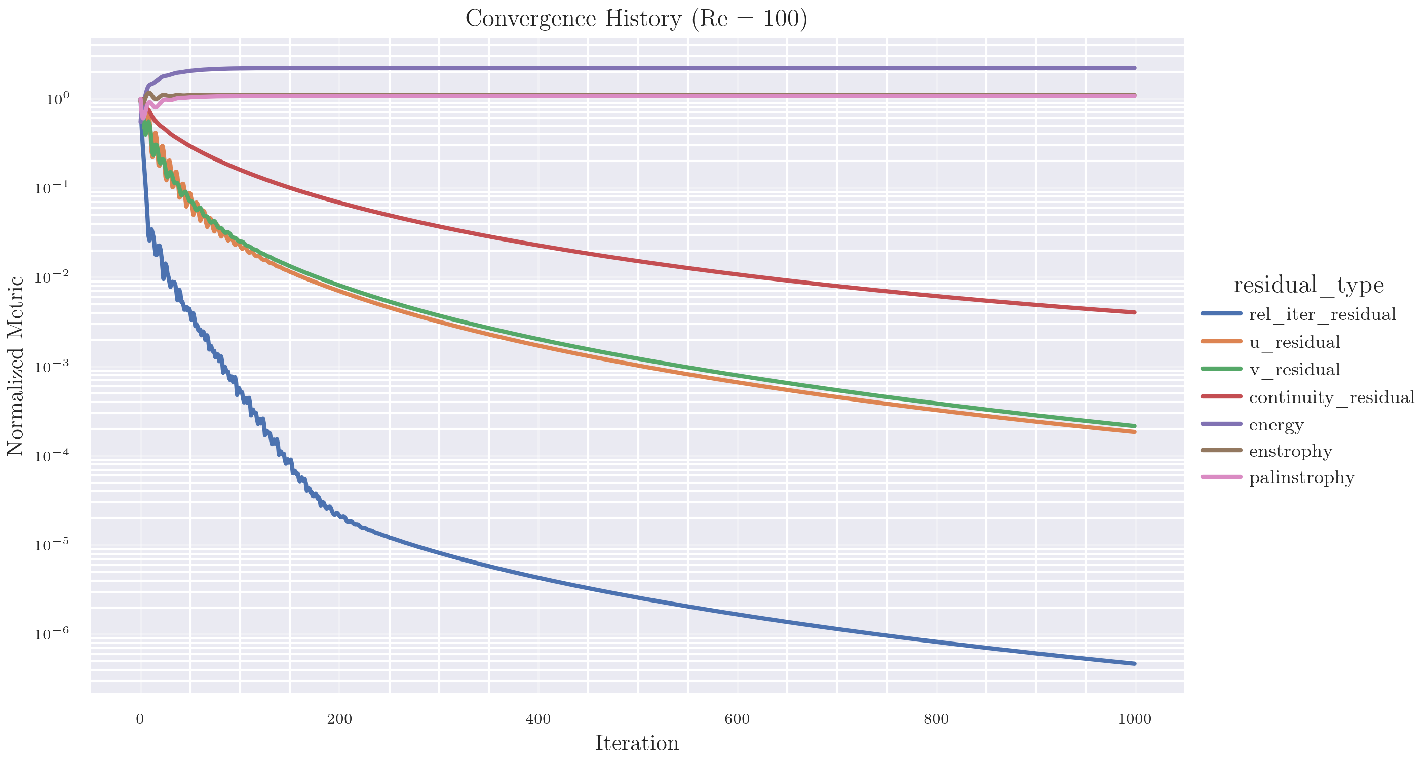
Convergence plot saved to: /home/runner/work/02689-AdvancedNumericalAlgorithmP3/02689-AdvancedNumericalAlgorithmP3/figures/FV-Solver/convergence_Re100.pdf
  ✓ Convergence saved

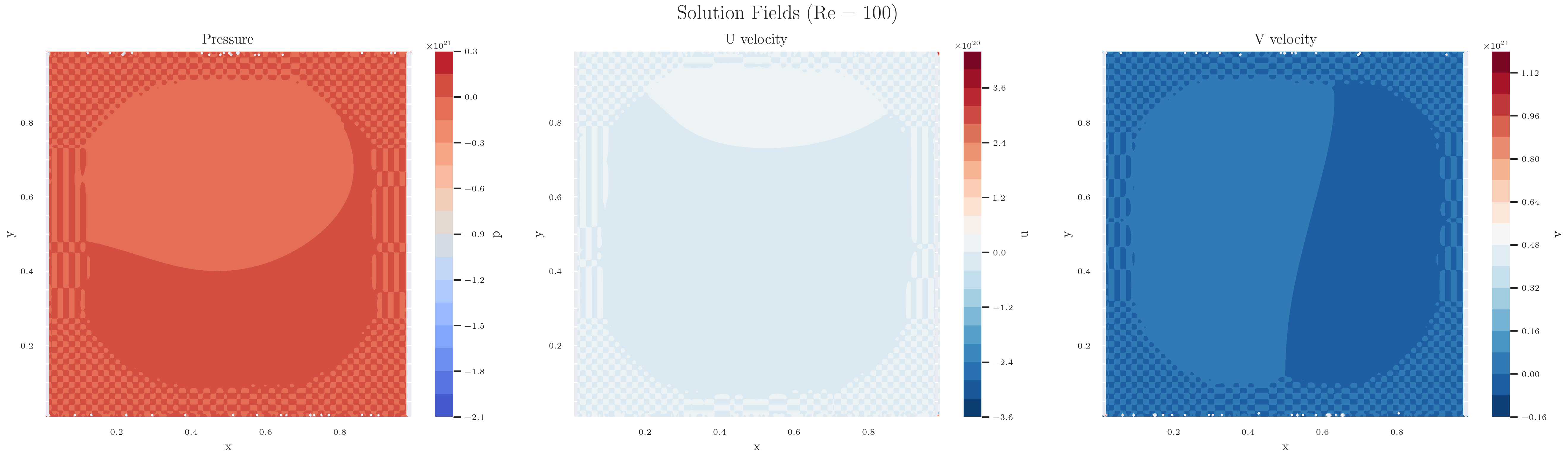
Solution Fields

Generate combined plot with pressure, u velocity, and v velocity fields.

plotter.plot_fields(output_path=fig_dir / f"fields_{Re_str}.pdf")
print("  ✓ Fields saved")

/home/runner/work/02689-AdvancedNumericalAlgorithmP3/02689-AdvancedNumericalAlgorithmP3/.venv/lib/python3.11/site-packages/scipy/interpolate/_polyint.py:850: RuntimeWarning: invalid value encountered in dot
  p = np.dot(c, self.yi) / np.sum(c, axis=-1)[..., np.newaxis]
Fields plot saved to: /home/runner/work/02689-AdvancedNumericalAlgorithmP3/02689-AdvancedNumericalAlgorithmP3/figures/FV-Solver/fields_Re100.pdf
  ✓ Fields saved

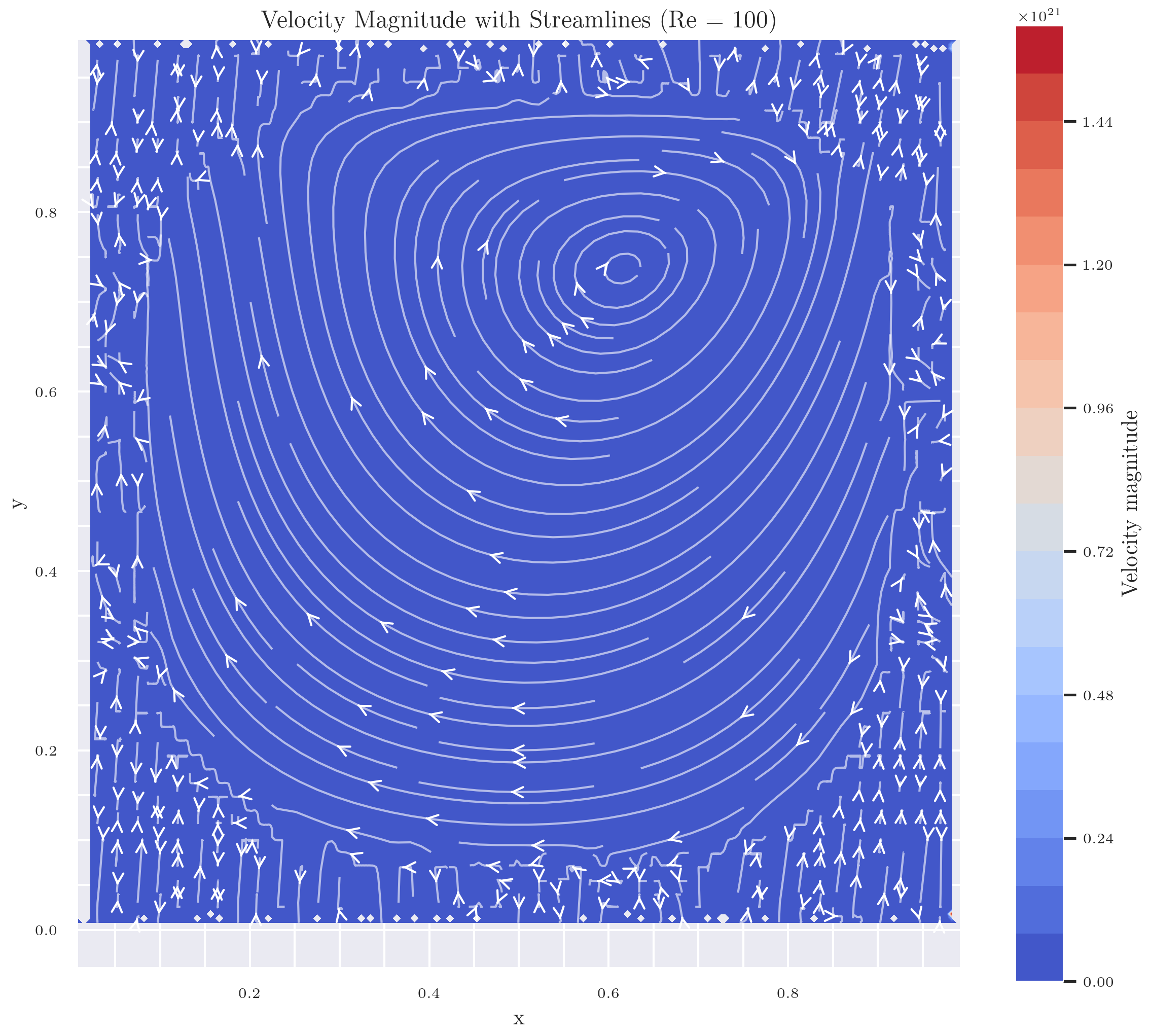
Velocity Magnitude with Streamlines

Velocity magnitude with streamlines overlaid

plotter.plot_streamlines(output_path=fig_dir / f"streamlines_{Re_str}.pdf")
print("  ✓ Streamlines saved")

/home/runner/work/02689-AdvancedNumericalAlgorithmP3/02689-AdvancedNumericalAlgorithmP3/.venv/lib/python3.11/site-packages/scipy/interpolate/_polyint.py:850: RuntimeWarning: invalid value encountered in dot
  p = np.dot(c, self.yi) / np.sum(c, axis=-1)[..., np.newaxis]
Streamlines plot saved to: /home/runner/work/02689-AdvancedNumericalAlgorithmP3/02689-AdvancedNumericalAlgorithmP3/figures/FV-Solver/streamlines_Re100.pdf
  ✓ Streamlines saved